NeurIPS 2026

SENSE: Semantic Neural Speech Synthesis
from Brain Dynamics via Spatial Graph Encoding

Jisoo Park¹*, Seonghak Lee¹, Hyojin Park², Junseok Kwon¹†

¹Chung-Ang University, South Korea · ²University of Birmingham, United Kingdom

susiehome@cau.ac.kr

* Work done during a research visit to the University of Birmingham. † Corresponding author.

🔊 Audio samples 📊 Results 💻 Code

SENSE overview animation — SENSE reads EEG recorded while a person listens, encodes it over the electrode geometry of the scalp, aligns that representation with a frozen CLIP text embedding on congruent trials only, and synthesizes the speech waveform. At inference only EEG is used.

Channel importance across the scalp for prior work and SENSE — **Figure 1.** EEG recorded during speech perception carries acoustic, sensorimotor, and lexical-semantic information distributed across the scalp. Prior work yields channel patterns with no clear anatomical structure (left). SENSE recovers attribution aligned with all three functional regions (right).

Abstract

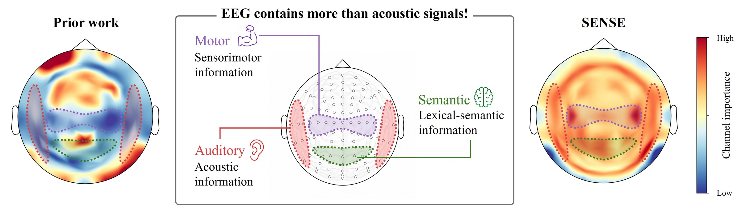
Existing EEG-to-speech approaches formulate the task as acoustic reconstruction, optimizing waveform fidelity while ignoring whether the generated speech preserves semantic content. We argue that EEG signals carry semantic as well as acoustic information, and that two limitations follow from the acoustic-only framing.

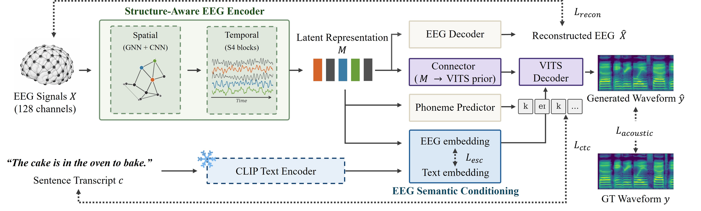
First, prior encoders treat the 128 electrodes as unordered feature dimensions, ignoring their spatial relationships. Second, they use the N400 corpus in a paradigm-agnostic manner, although the corpus is built around a congruency distinction designed to isolate semantic processing.

SENSE addresses both. A graph-based encoder models the electrodes over their scalp geometry, and EEG Semantic Conditioning (ESC) aligns the EEG latent with a frozen CLIP text embedding using congruent trials only. On the N400 dataset, SENSE outperforms prior methods on both acoustic and semantic metrics, with the largest gains on unseen participants.

Audio samples

Speech generated from EEG alone

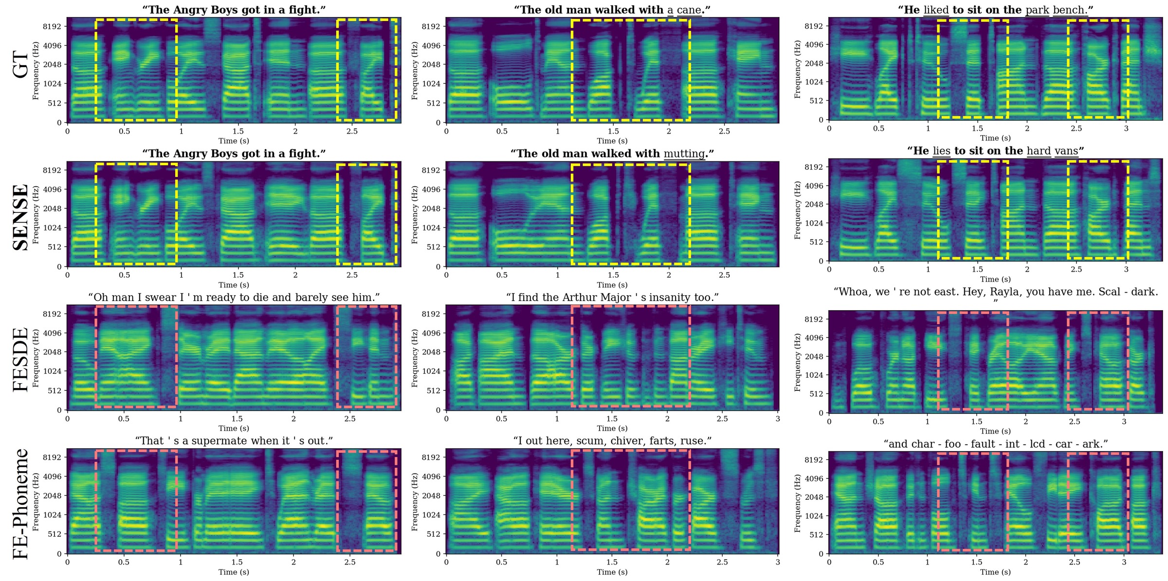
All samples come from the unseen-subject split. Generation is conditioned on EEG only, without text or guided sampling. Transcriptions are produced by Whisper-large, with words matching the stimulus shown in bold.

These are best-scoring examples.

“The old man walked with a cane.”

sub-24 · unseen subject · WER 29%

GT

SENSE

Whisper on SENSE output: “The old man walked with mutting.”

“On one hand I have five fingers.”

sub-23 · unseen subject · WER 29%

GT

SENSE

Whisper on SENSE output: “On one hand, I have five ears.”

“He liked to sit on the park bench.”

sub-24 · unseen subject · WER 38%

GT

SENSE

Whisper on SENSE output: “He lies to sit on the hard vans.”

“The angry boys got in a fight.”

sub-23 · unseen subject · WER 43%

GT

SENSE

Whisper on SENSE output: “The Angry Boys got in the fight.”

“He shut the door.”

sub-23 · unseen subject · WER 50%

GT

SENSE

Whisper on SENSE output: “He shust the poor.”

“He wore a cast because his arm broke.”

sub-24 · unseen subject · WER 50%

GT

SENSE

Whisper on SENSE output: “He wore a bass, he does his arm up”

Method

Structure-aware encoding and semantic conditioning

SENSE training pipeline — **Figure 2.** EEG is encoded into a latent representation and mapped to the prior of a VITS speech decoder. Solid arrows indicate the forward data flow, dashed arrows indicate loss supervision. At inference the EEG decoder, phoneme predictor, and CLIP encoder are discarded, and only EEG is required.

Graph-based spatial encoder. The 128 electrodes are represented as graph nodes with 3D BioSemi coordinates, connected by a fixed adjacency built from a Gaussian kernel over pairwise distances. Two residual graph-convolution layers mix information spatially. A parallel CNN branch preserves channel-specific detail that node averaging would otherwise attenuate, and a learnable scalar gate combines the two branches.
EEG Semantic Conditioning. The EEG latent is projected into the decoder conditioning space and aligned with a frozen CLIP text embedding under a cosine loss restricted to congruent trials, where the neural response reflects coherent semantic processing of the target word. Incongruent trials still contribute to the acoustic and phoneme objectives.
Conditioning bridge. During training the decoder is conditioned on one of three sources with roughly equal probability: the EEG-derived vector, the CLIP text embedding, or a learnable null embedding. This keeps the EEG vector in distribution when text conditioning is unavailable at inference.

Results

Comparison with prior methods

Three test conditions on the N400 corpus: held-out sentences (Audio), held-out participants (Subject), and held-out both. Semantic metrics are computed on congruent trials only. All results are averaged over five seeds.

Model	Split	MCD ↓	Mel-Corr ↑	STOI ↑	WER ↓	BERT-R ↑	CLIP-Sim ↑
FESDE	Both	11.80 ±0.12	19.87 ±1.97	0.2785	1.2186	0.0381	0.7557
FE-Phoneme	Both	10.52 ±0.08	28.29 ±1.34	0.3979	1.1610	0.0428	0.7509
SENSE	Both	10.44 ±0.10	31.18 ±0.60	0.3996	1.0186	0.0852	0.7654
FESDE	Audio	11.71 ±0.04	19.14 ±0.47	0.2792	1.2125	0.0289	0.7601
FE-Phoneme	Audio	10.73 ±0.06	26.53 ±0.30	0.3918	1.1360	0.0602	0.7554
SENSE	Audio	10.44 ±0.01	28.50 ±0.24	0.4039	1.0375	0.0959	0.7601
FESDE	Subject	11.73 ±0.04	18.70 ±0.29	0.2744	1.2171	0.0269	0.7587
FE-Phoneme	Subject	10.65 ±0.02	26.90 ±0.08	0.3806	1.1231	0.0564	0.7555
SENSE	Subject	9.928 ±0.03	32.07 ±0.14	0.4126	0.9948	0.1088	0.7647

SENSE outperforms both baselines across all splits and metrics. The margin is largest on the unseen-subject split, indicating that the learned representations generalize across participants rather than relying on subject-specific cues. Absolute WER remains near 1.0 for all methods, so intelligibility-level reconstruction from EEG remains an open challenge.

Qualitative comparison of generated speech — **Figure 3.** Mel-spectrograms and Whisper-large transcriptions for ground truth, SENSE, FESDE, and FE-Phoneme. Words matching the ground truth are shown in bold, semantically or phonetically similar words are underlined.

Cross-subject generalization

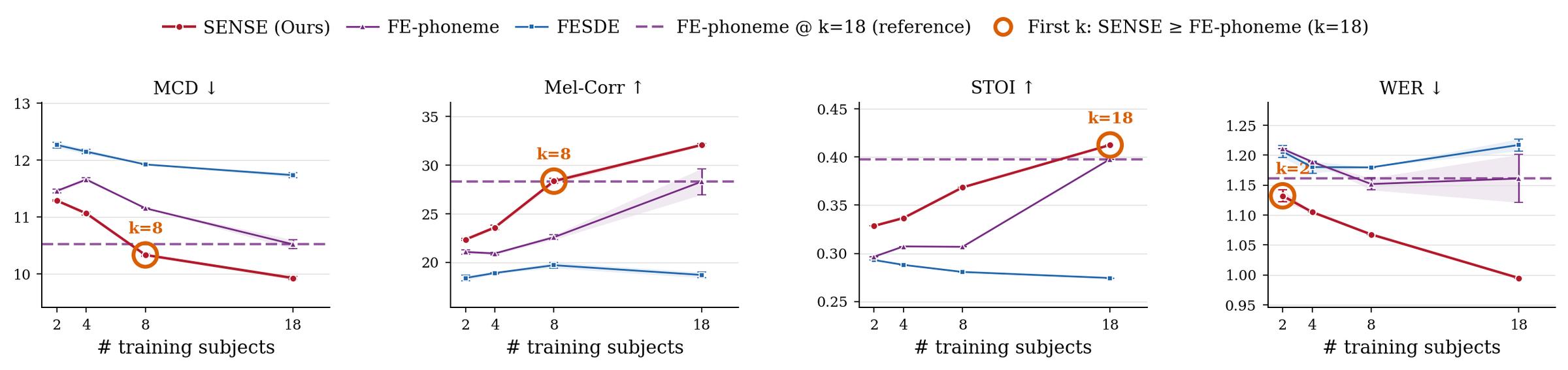
Scaling the number of training subjects

Models are trained on k participants and evaluated on a fixed held-out pair. The dashed line marks the strongest baseline trained on all 18 subjects. SENSE exceeds that reference on WER at k=2, and matches it on MCD and Mel-Correlation by k=8.

Scaling with the number of training subjects — **Figure 4.** Performance for k in {2, 4, 8, 18}, evaluated on the held-out pair (sub-23, sub-24). Shaded regions show ±1 std over 5 seeds. Orange circles mark the smallest k at which SENSE first matches or exceeds the 18-subject baseline. Since evaluation is on unseen participants, these results reflect cross-subject generalization rather than in-distribution scaling.

Ablation

Component ablation

Each row removes one component from the full model. Removing ESC degrades the semantic metrics, while removing CTC produces the largest increase in WER, indicating that phoneme-level supervision also preserves intelligibility.

Model	Ch.Att	GNN	Skip	CTC	ESC	MCD ↓	Mel-Corr ↑	STOI ↑	WER ↓	BERT-R ↑	CLIP-Sim ↑
SENSE	✓	✓	✓	✓	✓	9.93 ±0.03	32.07 ±0.14	0.4126	0.9948	0.1088	0.7647
w/o ESC	✓	✓	✓	✓	✗	10.34 ±0.03	29.43 ±0.27	0.4016	1.0323	0.0763	0.7601
w/ shuffled ESC	✓	✓	✓	✓	shuf.	10.38 ±0.04	29.25 ±0.28	0.4002	1.0385	0.0721	0.7595
w/o CTC	✓	✓	✓	✗	✓	10.50 ±0.01	27.24 ±0.27	0.3721	1.0488	0.0588	0.7624
w/o CNN Skip	✓	✓	✗	✓	✓	10.40 ±0.01	29.64 ±0.25	0.3970	1.0306	0.0724	0.7579
w/o GNN	✓	✗	✗	✓	✓	10.11 ±0.02	29.54 ±0.22	0.3951	1.0355	0.0788	0.7577
w/o Ch.Att	✗	✓	✓	✓	✓	10.24 ±0.01	29.08 ±0.16	0.4046	1.0170	0.0926	0.7639

ESC depends on correct semantic targets. Permuting the CLIP targets within each batch, while keeping the same loss and conditioning bridge, lowers BERT-R to 0.072, slightly below removing ESC entirely (0.076). The gain therefore comes from genuine EEG-semantic correspondence rather than auxiliary supervision alone.
Anatomy-derived adjacency outperforms learned graphs. Compared against GAT-learned edges, fully-connected, and random adjacency, the fixed BioSemi topology is best on every metric (WER 0.995 against 1.018, 1.095, and 1.081). Learning the graph from only 7,200 training pairs is under-constrained, while removing structure entirely is more harmful.
CLIP is the strongest alignment target. CLIP reaches BERT-R 0.109, ahead of text-only SBERT (0.094) and CLAP (0.092), despite CLAP being trained for audio-language alignment. A likely explanation is that N400 stimuli often involve concrete, image-able nouns, for which CLIP image-text pretraining provides more discriminative semantic structure.
ESC complements rather than replaces the encoder. Adding ESC to FESDE and FE-Phoneme improves both (BERT-R 0.045 and 0.070), but neither reaches SENSE.

EEG-text similarity matrices across semantic encoders — **Figure 6.** Cosine similarity between mean EEG embeddings (rows) and text embeddings (columns) for matched words. Stronger word-specific alignment appears as a brighter diagonal, and Δ is the gap between diagonal and off-diagonal means. CLIP shows the brightest diagonal and the largest gap.

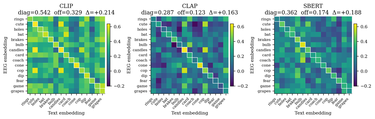
Analysis

Channel attribution

The channel attention gate is initialized with a positive bias on auditory-related electrodes and zero elsewhere. No prior is placed on sensorimotor or centro-parietal regions. After training, the auditory-prior channels are modestly down-weighted while central electrodes (C3, C4) gain importance, so the resulting pattern emerges from training rather than design.

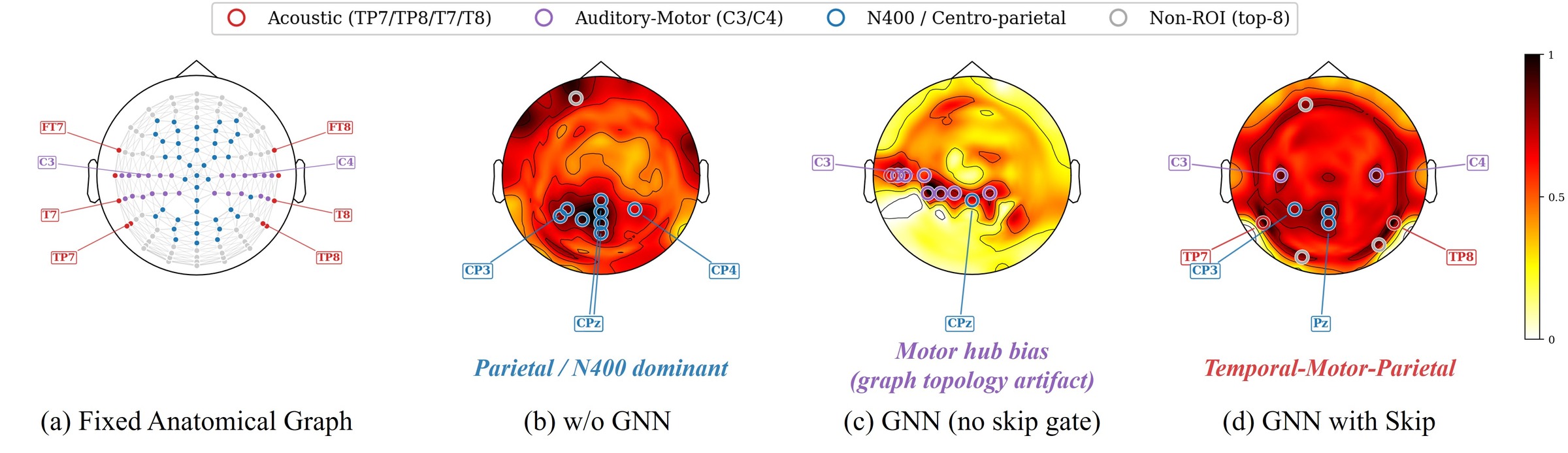
ESC attribution across encoder variants — **Figure 7.** Per-channel gradient magnitude of the EEG-CLIP alignment, normalized per model. (b) Without GNN: centro-parietal concentration consistent with the N400 response. (c) GNN without skip connection: emphasis shifts to central hub electrodes, a topology artifact of dense connectivity. (d) Full SENSE: a distributed pattern over temporal-auditory (TP7, TP8), motor (C3, C4), and centro-parietal (CPz) regions.

The prominence of C3 and C4 is consistent with prior findings that speech perception engages sensorimotor cortex during passive listening. We treat these maps as model-internal diagnostics rather than evidence of neural sources, given the known limitations of saliency-based attribution.

SENSE: Semantic Neural Speech Synthesisfrom Brain Dynamics via Spatial Graph Encoding

Speech generated from EEG alone

Structure-aware encoding and semantic conditioning

Comparison with prior methods

Scaling the number of training subjects

Component ablation

Channel attribution

SENSE: Semantic Neural Speech Synthesis
from Brain Dynamics via Spatial Graph Encoding